BRDF

The BRDF, or Bidirectional Reflective Distribution Function is a function that takes as input the incoming (light) direction $\omega_i$, the outgoing (view) direction $\omega_o$, the surface normal $n$ and a surface parameter a that represents the microsurface’s roughness. The BRDF approximates how much each individual light ray $\omega_i$ contributes to the final reflected light of an opaque surface given its material properties. For instance, if the surface has a perfectly smooth surface (like a mirror) the BRDF function would return 0.0 for all incoming light rays $\omega_i$ except the one ray that has the same (reflected) angle as the outgoing ray $\omega_o$ at which the function returns 1.0.

A BRDF approximates the material’s reflective and refractive properties based on the previously discussed microfacet theory. For a BRDF to be physically plausible it has to respect the law of energy conservation i.e. the sum of reflected light should never exceed the amount of incoming light. Technically, Blinn-Phong is considered a BRDF taking the same $\omega_i$ and $\omega_o$ as inputs. However, Blinn-Phong is not considered physically based as it doesn’t adhere to the energy conservation principle. There are several physically based BRDFs out there to approximate the surface’s reaction to light. However, almost all real-time render pipelines use a BRDF known as the Cook-Torrance BRDF.

The Cook-Torrance BRDF contains both a diffuse and specular part:

$$f_r = k_d f_{lambert} + k_s f_{cook-torrance}$$

Diffuse Part

Here kd is the earlier mentioned ratio of incoming light energy that gets refracted with ks being the ratio that gets reflected. The left side of the BRDF states the diffuse part of the equation denoted here as flambert. This is known as Lambertian diffuse similar to what we used for diffuse shading which is a constant factor denoted as:

$$f_{lambert} = \frac{c}{\pi}$$

With c being the albedo or surface color (think of the diffuse surface texture). The divide by pi is there to normalize the diffuse light as the earlier denoted integral that contains the BRDF is scaled by $\pi$

You might wonder how this Lambertian diffuse relates to the diffuse term we’ve been using before: the surface color multiplied by the dot product between the surface’s normal and the light direction. The dot product is still there, but moved out of the BRDF as we find $n \cdot \omega_i$ at the end of the $L_o$ integral.

There exist different equations for the diffuse part of the BRDF which tend to look more realistic, but are also more computationally expensive. As concluded by Epic Games however, the Lambertian diffuse is sufficient enough for most real-time rendering purposes.

Specluar Part

The specular part of the BRDF is a bit more advanced and is described as:

$$f_{cook-torrance} = \frac{DFG}{4(\omega_o \cdot n)(\omega_i \cdot n)}$$

he Cook-Torrance specular BRDF consists of three functions and a normalization factor in the denominator. Each of the D, F and G symbols represent a type of function that approximates a specific part of the surface’s reflective properties. These are defined as the normal Distribution function, the Fresnel equation and the Geometry function:

• Normal distribution function: approximates the amount the surface’s microfacets are aligned to the halfway vector influenced by the roughness of the surface; this is the primary function approximating the microfacets.
• Geometry function: describes the self-shadowing property of the microfacets. When a surface is relatively rough the surface’s microfacets can overshadow other microfacets thereby reducing the light the surface reflects.
• Fresnel equation: The Fresnel equation describes the ratio of surface reflection at different surface angles.

Normal distribution function

The normal distribution function D statistically approximates the relative surface area of microfacets exactly aligned to the (halfway) vector $h$. There are a multitude of NDFs defined that statistically approximate the general alignment of the microfacets given some roughness parameter and the one we’ll be using is known as the Trowbridge-Reitz GGX:

$$NDF_{GGX}(n,h,\alpha) = \frac{\alpha^2}{\pi ((n \cdot h)^2(\alpha^2 - 1) + 1)^2}$$

Here $h$ is the halfway vector to measure against the surface’s microfacets, with a being a measure of the surface’s roughness. If we take $h$ as the halfway vector between the surface normal and light direction over varying roughness parameters we get the following visual result:

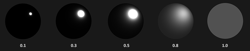
When the roughness is low (thus the surface is smooth) a highly concentrated number of microfacets are aligned to halfway vectors over a small radius. Due to this high concentration the NDF displays a very bright spot. On a rough surface however, where the microfacets are aligned in much more random directions, you’ll find a much larger number of halfway vectors h somewhat aligned to the microfacets, but less concentrated giving us the more grayish results.

In GLSL code the Trowbridge-Reitz GGX normal distribution function would look a bit like this:

float NormalDistributionFunction(float NoH, float Roughness)
{
    float a = Roughness * Roughness;
    float a2 = a * a;
    float NdotH = max(NoH, 0.0f);
    float NdotH2 = NdotH * NdotH;

    float nom = a2;
    float denom = (NdotH2 * (a2 - 1.0) + 1.0);
    denom = 3.141592 * denom * denom;

    return nom / denom;
}

Geometry function

The geometry function statistically approximates the relative surface area where its micro surface-details overshadow each other causing light rays to be occluded.

Similar to the NDF, the Geometry function takes a material’s roughness parameter as input with rougher surfaces having a higher probability of overshadowing microfacets. The geometry function we will use is a combination of the GGX and Schlick-Beckmann approximation known as Schlick-GGX:

$$G_{schlickGGX}(n,v,k) = \frac{n \cdot v}{(n \cdot v)(1-k) + k}$$

Here $k$ is a remapping of α based on whether we’re using the geometry function for either direct lighting or IBL lighting:

$$k_{direct} = \frac{(\alpha + 1)^2}{8}$$ $$k_{IBL} = \frac{\alpha^2}{2}$$

Note that the value of $\alpha$ might differ based on how your engine translates roughness to $\alpha$. In the following tutorials we’ll extensively discuss how and where this remapping becomes relevant.

To effectively approximate the geometry we need to take account of both the view direction (geometry obstruction) and the light direction vector (geometry shadowing). We can take both into account using Smith’s method:

$$G(n,v,l,k) = G_{sub}(n,v,k)G_{sub}(n,l,k)$$

Using Smith’s method with Schlick-GGX as $G_{sub}$ gives the following visual appearance over varying roughness R:

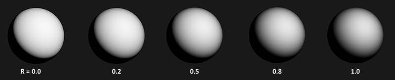
The geometry function is a multiplier between [0.0, 1.0] with white or 1.0 measuring no microfacet shadowing and black or 0.0 complete microfacet shadowing.

In GLSL the geometry function translates to the following code:

float GeometrychlickGGX(float NoV, float k)
{
    float nom = NoV;
    float denom = NoV * (1.0 - k) + k;

    return nom / denom;
}

float GeometryFunction(vec3 N, vec3 V, vec3 L, float Roughness)
{
    float k = pow(Roughness + 1, 2) / 8.0f;
    float NoV = max(dot(N, V), 0.0);
    float NoL = max(dot(N, L), 0.0);
    float ggx1 = GeometrychlickGGX(NoV, k);
    float ggx2 = GeometrychlickGGX(NoL, k);

    return ggx1 * ggx2;
}

Fresnel equation

The Fresnel equation (pronounced as Freh-nel) describes the ratio of light that gets reflected over the light that gets refracted, which varies over the angle we’re looking at a surface. The moment light hits a surface, based on the surface to view angle the Fresnel equation tells us the percentage of light that gets reflected. From this ratio of reflection and the energy conservation principle we can directly obtain the refracted portion of light from its remaining energy.

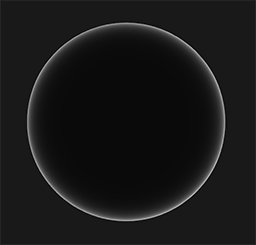
Every surface or material has a level of base reflectivity when looking straight at its surface, but when looking at the surface from an angle all reflections become more apparent compared to the surface’s base reflectivity. You can check this for yourself by looking at your presumably wooden/metallic desk which has a certain level of base reflectivity from a perpendicular view angle, but by looking at your desk from an almost 90 degree angle you’ll see the reflections become much more apparent. All surfaces theoretically fully reflect light if seen from perfect 90-degree angles. This phenomenon is known as Fresnel and is described by the Fresnel equation.

The Fresnel equation is a rather complex equation, but luckily the Fresnel equation can be approximated using the Fresnel-Schlick approximation:

$$F_{schlick}(h,v,F_0) = F_0 + (1 - F_0)(1 - (h \cdot v))^5$$

$F_0$ represents the base reflectivity of the surface, which we calculate using something called the indices of refraction or IOR and as you can see on a sphere surface, the more we look towards the surface’s grazing angles (with the halfway-view angle reaching 90 degrees) the stronger the Fresnel and thus the reflections:

There are a few subtleties involved with the Fresnel equation. One is that the Fresnel-Schlick approximation is only really defined for dielectric or non-metal surfaces. For conductor surfaces (metals) calculating the base reflectivity using their indices of refraction doesn’t properly hold and we need to use a different Fresnel equation for conductors altogether. As this is inconvenient we further approximate by pre-computing the surface’s response at normal incidence ($F0$) (at a 0 degree angle as if looking directly onto a surface) and interpolate this value based on the view angle as per the Fresnel-Schlick approximation such that we can use the same equation for both metals and non-metals.

These specific attributes of metallic surfaces compared to dielectric surfaces gave rise to something called the metallic workflow where we author surface materials with an extra parameter known as metalness that describes whether a surface is either a metallic or a non-metallic surface.

Theoretically the metalness of a surface is binary: it’s either a metal or it isn’t; it can’t be both. However, most render pipelines allow configuring the metalness of a surface linearly between 0.0 and 1.0. This is mostly because of the lack of material texture precision to describe for instance a surface having small dust/sand-like particles/scratches over a metallic surface. By balancing the metalness value around these small non-metallic like particles/scratches we get visually pleasable results.

vec3 FresnelEquation(vec3 N, vec3 V, vec3 F)
{
    float NoV = dot(N, V);
    vec3 res = F + (vec3(1.0f) - F) * pow(1.0f - NoV, 5);
    return res;
}

Cook-Torrance reflectance equation

With every component of the Cook-Torrance BRDF described we can include the physically based BRDF into the now final reflectance equation:

$$L_o(p,w_o) = \int_\pi(k_d \frac{c}{\pi} + k_s \frac{DFG}{4(w_o \cdot n)(w_i \cdot n)})L_i(p,w_i)n \cdot w_idw_i$$

This equation is however not fully mathematically correct. You may remember that the Fresnel term $F$ represents the ratio of light that gets reflected on a surface. This is effectively our ratio $k_s$, meaning the specular part of the reflectance equation implicitly contains the reflectance ratio $k_s$. Given this, our final final reflectance equation becomes:

$$L_o(p,w_o) = \int_\pi(k_d \frac{c}{\pi} + \frac{DFG}{4(w_o \cdot n)(w_i \cdot n)})L_i(p,w_i)n \cdot w_idw_i$$

This equation now completely describes a physically based render model that is generally recognized as what we commonly understand as physically based rendering or PBR. Don’t worry if you didn’t yet completely understand how we’ll need to fit all the discussed mathematics together in code. In the next tutorials, we’ll explore how to utilize the reflectance equation to get much more physically plausible results in our rendered lighting and all the bits and pieces should slowly start to fit together.

Reference

Learn OpenGL PBR Theory